38 excel pivot table 2 row labels

Pivot Table adding "2" to value in answer set 1) Right click your pivot table -> Pivot table options -> Data -> Change "Number of items to retain per field" to NONE 2) Wipe all rows in your data source except for the headers 3) Refresh the pivot table 4) Save, and close all instances of Excel 5) Reopen the file, and paste your data 6) Refresh the pivot table How do you regroup in a pivot table? - Terasolartisans.com Drag and drop a field into the "Row Labels" area. ... You can group rows and columns in your Excel pivot table. To create a grouping, select the items that you want to group, right-click the pivot table, and then choose Group from the shortcut menu that appears. Excel creates a new grouping, which it names in numerical order starting with ...

PivotTable options Use the PivotTable Options dialog box to control various settings for a PivotTable.. Name Displays the PivotTable name.To change the name, click the text in the box and edit the name. Layout & Format. Layout section. Merge and center cells with labels Select to merge cells for outer row and column items so that you can center the items horizontally and vertically.

Excel pivot table 2 row labels

How do you collapse rows in a pivot table ... How do I move a row label to a column in a pivot table? Use Menu Commands to Move Label To move a pivot table label to a different position in the list, you can use commands in the right-click menu: Right-click on the label that you want to move. Click the Move command. Click one of the Move subcommands, such as Move [item name] Up. pivot table - How to extract the full row label from Excel ... I know that I can go to PivotTable Tools > Design > Report Layout > Show in Tabular Form and then Repeat All Item Labels and then use a simple formula to get the full row label into a single cell, but I am trying to avoid changing the format of the PivotTable. Automatic Row And Column Pivot Table Labels - How To Excel ... Select the data set you want to use for your table The first thing to do is put your cursor somewhere in your data list Select the Insert Tab Hit Pivot Table icon Next select Pivot Table option Select a table or range option Select to put your Table on a New Worksheet or on the current one, for this tutorial select the first option Click Ok

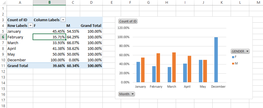
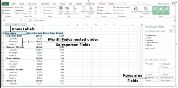
Excel pivot table 2 row labels. Excel Pivot Table with nested rows - Basic Excel Tutorial 2. Once you create your pivot table, add all the fields you need to analyze data. How to add the fields. Select the checkbox on each field name you desire in the field section. The selected fields are added to the Row Labels area in the layout section. You can drag a field you want from the field section to an area in the layout section. How to rename group or row labels in Excel PivotTable? 1. Click at the PivotTable, then click Analyze tab and go to the Active Field textbox. 2. Now in the Active Field textbox, the active field name is displayed, you can change it in the textbox. You can change other Row Labels name by clicking the relative fields in the PivotTable, then rename it in the Active Field textbox. How do I make multiple row labels in a pivot table? - idswater ... Feb 3, 2021 — Click anywhere in a pivot table to open the editor. Add data—Depending on where you want to add data, under Rows, Columns, or Values, click Add. Pivot Table Sort by second row label - Microsoft Community Ramz Aftab Replied on May 17, 2014 Here is how you can get the results: Place your cursor on Col. B data wherever Names are. Goto Home ribbon>Editing>Sort it in either way. Alternatively, you can Sort from Pivots settings. Ramz Aftab [ MOS 77-888/82 Excel Expert ] ramzaftab [at]gmail [.]com Report abuse Was this reply helpful?

ExtendOffice - Beste tools voor kantoorproductiviteit ExtendOffice - Beste tools voor kantoorproductiviteit Pivot Table "Row Labels" Header Frustration - Microsoft ... Hi Everyone please help I can't change my headers from Row Labels in a Pivot Table. Using Excel 365 Design the layout and format of a PivotTable Click anywhere in the PivotTable. This displays the PivotTable Tools tab on the ribbon. On the Options tab, in the PivotTable group, click Options. In the PivotTable Options dialog box, click the Layout & Format tab, and then under Layout, select or clear the Merge and center cells with labels check box. How to make row labels on same line in pivot table? Make row labels on same line with setting the layout form in pivot table As we all know, the pivot table has several layout form, the tabular form may help us to put the row labels next to each other. Please do as follows: 1. Click any cell in your pivot table, and the PivotTable Tools tab will be displayed. 2.

How to Use Excel Pivot Table Label Filters The item is immediately hidden in the pivot table. Quickly Hide All But a Few Items. You can use a similar technique to hide most of the items in the Row Labels or Column Labels. Select the pivot table items that you want to keep visible; Right-click on one of the selected items; In the pop-up menu, click Filter, then click Keep Only Selected ... Pivot table row labels in separate columns - Audit Excel So when you click in the Pivot Table and click on the DESIGN tab one of the options is the Report Layout. Click on this and change it to Tabular form. Your pivot table report will now look like the bottom picture and will be easier to use in other areas of the spreadsheet and in our opinion is also easier to read. Combining row labels in pivot table : excel - reddit The problem is some of the data represents the same thing but aren't identical so they get different rows. As an example if the row labels are salesman and some of the cells from the raw table have James Bond and others have bond, or JB. Each of these iteration gets its own row in the pivot table. Pivot table row labels side by side - Excel Tutorials You can copy the following table and paste it into your worksheet as Match Destination Formatting. Now, let’s create a pivot table ( Insert >> Tables >> Pivot Table) and check all the values in Pivot Table Fields. Fields should look like this. Right-click inside a pivot table and choose PivotTable Options…. Check data as shown on the image below.

Pivot Tables – excelhelpsblog

Combining two+ Columns to form one Row label column in ... Re: Combining two+ Columns to form one Row label column in Pivot Table Select a cell in your pivot table. Press Alt, then D, then P (i.e. in succession; not all at the same time), to call up the Pivot Table Wizard. Click "" button twice.

Excel Pivot Table Report - Sort Data in Row & Column Labels & in Values Area, use Custom Lists

How to Customize Your Excel Pivot Chart Data Labels - dummies The Data Labels command on the Design tab's Add Chart Element menu in Excel allows you to label data markers with values from your pivot table. When you click the command button, Excel displays a menu with commands corresponding to locations for the data labels: None, Center, Left, Right, Above, and Below. None signifies that no data labels should be added to the chart and Show signifies ...

How to repeat row labels for group in pivot table?

Repeat item labels in a PivotTable Right-click the row or column label you want to repeat, and click Field Settings. Click the Layout & Print tab, and check the Repeat item labels box. Make sure Show item labels in tabular form is selected. Notes: When you edit any of the repeated labels, the changes you make are applied to all other cells with the same label.

Repeat Pivot Table Labels in Excel 2010 - Excel Pivot TablesExcel Pivot Tables

Formula1, Formula2 appearing as row items in pivot table ... Formula1, Formula2 appearing as row items in pivot table where row labels previously were I was greeted by a spreadsheet that my wife was using that she had messed up. A table than previously showed date, time, address and hours , was now replaced by date, time, formula1, formula2....formula7 as the values in a column and then the duration.

Microsoft Office 2016 - IT Knowledge Base - Confluence

How to add side by side rows in excel pivot table ? | AnswerTabs You have to right-click on pivot table and choose the PivotTable options. Then swich to Display tab and turn on Classic PivotTable layout: Now the pivot table should look like this: As a next step, you have to modify the Field settings of the rows: In subtotals section choose None: The pivot table rows should be now placed next to each other:

Design your Pivot Table in Excel | Excel in Excel

How to repeat row labels for group in pivot table? In Excel, when you create a pivot table, the row labels are displayed as a compact layout, all the headings are listed in one column. Sometimes, you need to convert the compact layout to outline form to make the table more clearly. But in tphe outline layout, the headings will be displayed at the top of the group.

Excel Pivot Table Report - Sort Data in Row & Column Labels & in Values Area, use Custom Lists

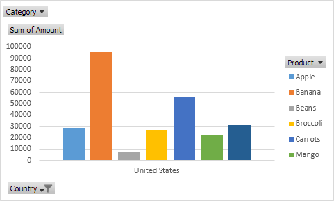
Multi-level Pivot Table in Excel (In Easy Steps) First, insert a pivot table. Next, drag the following fields to the different areas. 1. Country field to the Rows area. 2. Amount field to the Values area (2x). Note: if you drag the Amount field to the Values area for the second time, Excel also populates the Columns area. Pivot table: 3. Next, click any cell inside the Sum of Amount2 column. 4.

Excel Pivot Tables Explained • My Online Training Hub

pivot table how to combine 2 row labels - MrExcel Message Board Nov 06, 2013 · pivot table how to combine 2 row labels sdsurzh Nov 6, 2013 S sdsurzh Board Regular Joined Sep 27, 2009 Messages 248 Nov 6, 2013 #1 Hi, i am having the pivot table in the below format. my concern is how i can combine both A & AA together the source is from data connection and not from the excel.

Excel is more than a calculator! - Part 2 (Pivot Tables, Pivot Charts & Slicers) | PTR

get a row label from pivot table - Microsoft Tech Community Alternatively you may work with cube assuming you are at least on Excel 2010, as I remember it's the first which supports data model. Create PivotTable and after that convert it to cube formulas. Now you may take these formulas and convert it to form you need, for example. =CUBEVALUE( "ThisWorkbookDataModel", CUBEMEMBER("ThisWorkbookDataModel ...

Advanced Excel - Pivot Table Recommendations - Tutorial Desk

Pivot Table Row Labels In the Same Line - Beat Excel! First make a pivot table with required fields. Arrange the fields as shown in left picture. Your initial table will look like right picture. Now click on "Error Code" and access field settings. First check "None" option in "Subtotals & Filters" tab to disable totals after every row.

Repeat Pivot Table Labels in Excel 2010 - Excel Pivot TablesExcel Pivot Tables

excel - Custom row labels in PivotTable - Stack Overflow If you go the pivot table data and right click you can change the value field settings to give a custom name to a row/series but I do not know about individual data points. path: pivot table data => right click => select Field Settings => edit custom name. It does not look like it modifies the raw data (before pivot table).

33 Pivot Table Blank Row Label - Labels Database 2020

Automatic Row And Column Pivot Table Labels - How To Excel ... Select the data set you want to use for your table The first thing to do is put your cursor somewhere in your data list Select the Insert Tab Hit Pivot Table icon Next select Pivot Table option Select a table or range option Select to put your Table on a New Worksheet or on the current one, for this tutorial select the first option Click Ok

How to Create Pivot Table in Excel

pivot table - How to extract the full row label from Excel ... I know that I can go to PivotTable Tools > Design > Report Layout > Show in Tabular Form and then Repeat All Item Labels and then use a simple formula to get the full row label into a single cell, but I am trying to avoid changing the format of the PivotTable.