42 pivot table excel multiple row labels
Remove PivotTable Duplicate Row Labels [SOLVED] Re: Remove PivotTable Duplicate Row Labels Sometimes when the cells are stored in different formats within the same column in the raw data, they get duplicated. Also, if there is space/s at the beginning or at the end of these fields, when you filter them out they look the same, however, when you plot a Pivot Table, they appear as separate headers. Excel Pivot Table with multiple columns of data and each data … 17/04/2019 · Then I made multiple Pivot Tables, filling the Columns and Values Pivot Table Fields with one Category of each of your categories. This will produce a Pivot Table with 3 rows. The first row will read Column Labels with a filter dropdown. The second row will read all the possible values of the column. The third row will be the count of each ...
row - Excel pivot table: How to transpose multiple value in column to a ... Here's the pivot table I have in excel: I have a list of website with their emails address. Sometime you have one email per website, sometime you have 3 emails per website. I want to transpose the multiple emails I have for one website that are in column Email 1 into multiple field such as Email 1, Email 2, Email 3 for EACH corresponding websites.
Pivot table excel multiple row labels
Ranking to a Pivot Table with multiple Row Labels I have a pivot table with multiple Row Labels: Team and Player I then have a bunch of stat categories under Values, one of which is 'Pts' I have the table sorted by Pts, but I need a 'Ranking' column I created a second Pts column and used 'Show Values As - Rank Largest to Smallest', but it's not working. How to Use Excel Pivot Table Label Filters To change the Pivot Table option to allow multiple filters: Right-click a cell in the pivot table, and click PivotTable Options. Click the Totals & Filters tab Under Filters, add a check mark to 'Allow multiple filters per field.' Click OK Quick Way to Hide or Show Pivot Items Easily hide or show pivot table items, with the quick tip in this video. How to make row labels on same line in pivot table? Make row labels on same line with PivotTable Options You can also go to the PivotTable Options dialog box to set an option to finish this operation. 1. Click any one cell in the pivot table, and right click to choose PivotTable Options, see screenshot: 2.
Pivot table excel multiple row labels. How to Filter Multiple Values in Pivot Table – Excel Tutorials When we click OK, we will have only LeBron James selected in our Pivot Table:. Filter with Slicers. Another way to filter multiple values in Pivot Table is to use Slicers.We will create another Pivot Table with the same data. Then we will place player, team, and conference in rows fields and the sum of points, rebounds, assists in the values field. How can I make multiple pivot tables mimic the filters (report and row ... So I have multiple pivot tables on a single sheet in excel. I have a long list of months in the row labels. The report filter is filterable by names. All of the columns in the pivots are just sums of ... Browse other questions tagged vba excel pivot-table or ask your own question. The Overflow Blog The complete beginners guide to graph theory ... Repeat item labels in a PivotTable - support.microsoft.com Right-click the row or column label you want to repeat, and click Field Settings. Click the Layout & Print tab, and check the Repeat item labels box. Make sure Show item labels in tabular form is selected. Notes: When you edit any of the repeated labels, the changes you make are applied to all other cells with the same label. How to group time by hour in an Excel pivot table? Now the pivot table is added. Right-click any time in the Row Labels column, and select Group in the context menu. See screenshot: 5. In the Grouping dialog box, please click to highlight Hours only in the By list box, and click the OK button. See screenshot: Now the time data is grouped by hours in the newly created pivot table. See screenshot:
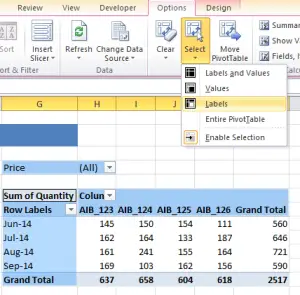
Excel Pivot Table Report - Clear All, Remove Filters, Select ... Excel Pivot Table Report - Clear All, Remove Filters, Select Mutliple Cells or Items, Move a Pivot Table. As applicable to Excel 2007 With the tools available in the Actions group of the 'Options' tab (under the 'Pivot Table Tools' tab on the ribbon), you can Clear a Pivot Table, Remove Filters, Select Multiple Cells or Items, and Move a Pivot Table report. How to add multiple fields into pivot table? - ExtendOffice After creating the pivot table, firstly, you should add the row label fields as your need, and leaving the value fields in the Choose fields to add to report list, see screenshot:< /p> 2 . Hold down the ALT + F11 keys to open the Microsoft Visual Basic for Applications window . How to repeat row labels for group in pivot table? - ExtendOffice Except repeating the row labels for the entire pivot table, you can also apply the feature to a specific field in the pivot table only. 1. Firstly, you need to expand the row labels as outline form as above steps shows, and click one row label which you want to repeat in your pivot table. 2. Excel Pivot Table Group: Step-By-Step Tutorial To Easily Group … Let's start by looking at the… Example Pivot Table And Source Data. This Pivot Tutorial is accompanied by an Excel workbook example. If you want to follow each step of the way and see the results of the processes I explain below, you can get immediate free access to this workbook by subscribing to the Power Spreadsheets Newsletter.. I use the following source data for all …
Pivot table - Wikipedia Pivot tables are not created automatically. For example, in Microsoft Excel one must first select the entire data in the original table and then go to the Insert tab and select "Pivot Table" (or "Pivot Chart"). The user then has the option of either inserting the pivot table into an existing sheet or creating a new sheet to house the pivot table. How to Filter Multiple Values in Pivot Table – Excel Tutorials Our Pivot Table now looks like this: Filter with Pivot Table Label Filters. Now we will clear all of our filters. To clear them all out at the same time, we will click anywhere on our Pivot Table, then go to PivotTable Analyze field >> Actions >> Clear Filters: Once we do that, we will go to our Pivot Table, go to a dropdown at the Row Labels ... How to Format Excel Pivot Table - Contextures Excel Tips 23/05/2022 · The pasted copy looks like the original pivot table, without the link to the source data. TOP . Keep Formatting in Excel Pivot Table. A pivot table is automatically formatted with a default style when you create it, and you can select a different style later, or add your own formatting. For example, in the pivot table shown below, colour has ... How to Format Excel Pivot Table - Contextures Excel Tips May 23, 2022 · Keep Formatting in Excel Pivot Table. A pivot table is automatically formatted with a default style when you create it, and you can select a different style later, or add your own formatting. For example, in the pivot table shown below, colour has been added to the subtotal rows, and column B is narrow.
Excel Tip-How To Quickly Select All Or Just Parts Of Your Pivot Table - How To Excel At Excel
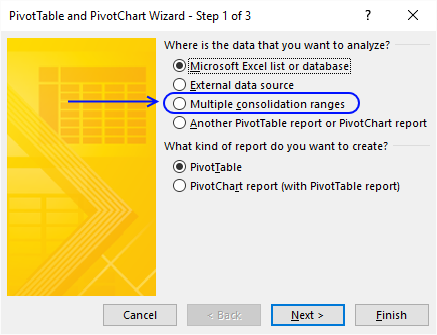
Excel Pivot Table Multiple Consolidation Ranges 15/11/2021 · Pivot Table from Multiple Consolidation Ranges. To open the PivotTable and PivotChart Wizard, select any cell on a worksheet, then press Alt+D, then press P. That shortcut is used because in older versions of Excel, the wizard was listed on the Data menu, as the PivotTable and PivotChart Report command. Click Multiple consolidation ranges, then click …
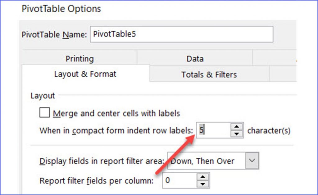
How to Increase Indent Row Labels in Pivot Table Compact Form - ExcelNotes
Pivot table row labels side by side - Excel Tutorials You can copy the following table and paste it into your worksheet as Match Destination Formatting. Now, let's create a pivot table ( Insert >> Tables >> Pivot Table) and check all the values in Pivot Table Fields. Fields should look like this. Right-click inside a pivot table and choose PivotTable Options…. Check data as shown on the image below.

filtering - Applying Multiple Value Filters in Excel Pivot - Stack Overflow
Pivot Table Multiple Row Labels? [SOLVED] - Excel Help Forum Is it possible to have two Row Labels showing in a Pivot Table, instead of one showing as a sub-category of the other. I have a spreadsheet that shows the status (Design, Development, Testing, Live), owner and engineer for software. I currently have to have two separate pivot tables: 1) showing count of software in each status for each owner.

excel - Extract Pivot Table Row Label (not value) - Stack Overflow
Excel Pivot Table Group: Step-By-Step Tutorial To Group Or ... In fact, as mentioned in Excel 2016 Pivot Table Data Crunching: Each time you create a new pivot table in Excel 2016, Excel automatically shares the pivot cache. Pivot Cache sharing has several benefits. Most notably, as I mention above, it reduces memory requirements and file size vs. the scenario where the Pivot Cache isn't shared.

How to Sort Pivot Table Row Labels, Column Field Labels and Data Values with Excel VBA Macro ...
How to make row labels on same line in pivot table in excel #ExcelMaster, #PivotTable, #ExcelHow to make row labels on same line in pivot table in excelHow to show multiple rows in pivot table in excel

Tutorial 2: Pivot Tables in Microsoft Excel: Tutorial 2: Pivot Tables in Microsoft Excel
multiple fields as row labels on the same level in pivot table Excel ... multiple fields as row labels on the same level in pivot table Excel 2016 I am using Excel 2016. I have data that lists product models along with relevant data and also production volumes by month. Part of the relevant data are about 5 common part columns with the part # that applies to each model under the appropriate column.

Pivot Tables for Excel - This is the Ultimate Guide (NEW)
Excel Pivot Table Report - Clear All, Remove Filters, Select … Pivot Table Options tab - Actions group Customizing a Pivot Table report: When you insert a Pivot Table, a blank Pivot Table report is created in the specified location, and the 'PivotTable Field List' Pane also appears which allows you to Add or Remove Fields, Move Fields to different Areas and to set Field Settings. The 'Options' and 'Design' tabs (under the 'PivotTable Tools' …

How to Sort Pivot Table Row Labels, Column Field Labels and Data Values with Excel VBA Macro ...
Help. How do I do multiple Value Filters on a pivot table row label ... Right-Click on your Row Label > Value Filters... If you have multiple value fields, you should be able to dropdown the listbox under "Show items for which". If you have more than one Row Field make sure that the Value Filter (your field name) title is at the correct level, as you can filter at different levels.
Discover Pivot Tables – Excel’s most powerful feature and also least known
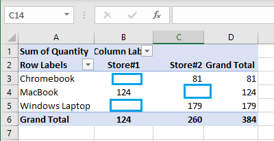
Multi-level Pivot Table in Excel (In Easy Steps) Below you can find the multi-level pivot table. Multiple Value Fields First, insert a pivot table. Next, drag the following fields to the different areas. 1. Country field to the Rows area. 2. Amount field to the Values area (2x). Note: if you drag the Amount field to the Values area for the second time, Excel also populates the Columns area.
How to repeat row labels for group in pivot table?
Pivot Table Row Labels In the Same Line - Beat Excel! It is a common issue for users to place multiple pivot table row labels in the same line. You may need to summarize data in multiple levels of detail while rows labels are side by side. In this post I'm going to show you how to do it. ... After creating a pivot table in Excel, you will see the row labels are listed in only one column. But, if ...
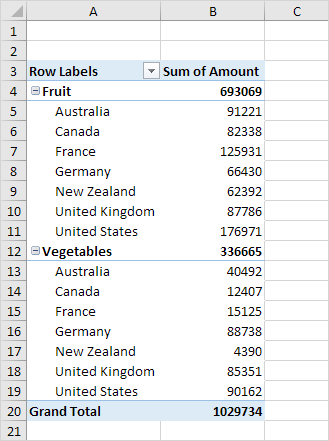
Multi-level Pivot Table in Excel - Easy Excel Tutorial
Excel tutorial: How to filter a pivot table with multiple filters To enable multiple filters per field, we need to change a setting in the pivot table options. Right-click in the pivot table and select PivotTable Options from the menu. then navigate to the Totals & Filters tab. There, under Filters, enable "allow multiple filters per field". Back in our pivot table, let's enable the Value Filter again ...
32 Pivot Table Blank Row Label - Labels For You
How to make row labels on same line in pivot table? Make row labels on same line with PivotTable Options You can also go to the PivotTable Options dialog box to set an option to finish this operation. 1. Click any one cell in the pivot table, and right click to choose PivotTable Options, see screenshot: 2.
Repeat Pivot Table Labels in Excel 2010 – Excel Pivot Tables
How to rename group or row labels in Excel PivotTable? 1. Click at the PivotTable, then click Analyze tab and go to the Active Field textbox. 2. Now in the Active Field textbox, the active field name is displayed, you can change it in the textbox. You can change other Row Labels name by clicking the relative fields in the PivotTable, then rename it in the Active Field textbox.

Excel For Mac Pivot Table Repeat Item Labels - foxprofit
How to Add Rows to a Pivot Table: 9 Steps (with Pictures) 15/02/2022 · You can use pivot tables in Excel and Google Sheets to group and organize data in a spreadsheet. Adding rows to a pivot table is as simple as dragging fields into the "Rows" area of your pivot table formatting panel. We'll show you how to add new rows to an existing pivot table in both Microsoft Excel and Google Sheets.

How to make row labels on same line in pivot table?
Excel Pivot Table Multiple Consolidation Ranges Nov 15, 2021 · Pivot Table from Multiple Consolidation Ranges To open the PivotTable and PivotChart Wizard, select any cell on a worksheet, then press Alt+D, then press P. That shortcut is used because in older versions of Excel, the wizard was listed on the D ata menu, as the P ivotTable and PivotChart Report command.

Pivot table row labels in separate columns • AuditExcel.co.za
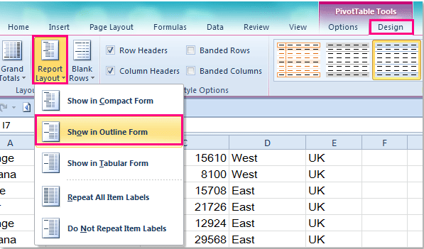
Pivot table row labels in separate columns • AuditExcel.co.za Our preference is rather that the pivot tables are shown in tabular form (all columns separated and next to each other). You can do this by changing the report format. So when you click in the Pivot Table and click on the DESIGN tab one of the options is the Report Layout. Click on this and change it to Tabular form.
Post a Comment for "42 pivot table excel multiple row labels"